Heads or Tails?

Question: How can Excel model the flip of a coin?

Lesson Goals: Understand the probability of tossing a coin. Review previous Excel skills.

New Skills: Excel functions RAND and INT. Arranging Excel worksheets and windows.

Old Skills: Copy and paste cells. Relative and absolute cell references.

Part A – Coin Tossing: The AVERAGE function

You’re going to flip a coin ten times and record the result in Excel. You will model the result of a coin flip using “0” for tails and “1” for heads.

If you record a great many coin flips as a 0 or 1 value, what does the value average out to? You can use the AVERAGE function to find out:

  1. Start Excel

  2. Save your workbook as “Coin Flips

  3. Click on cell A1 and enter:
        Coin Toss

  4. Click on cell A2

  5. Flip a coin, a real coin like a penny.

  6. If it’s heads, enter:
        1
    If it’s tails, enter:
        0

  7. Click on the next cell down

  8. Repeat steps 5-6 nine times, leaving you with ten total coin flips.

    Your worksheet should look something like the one to the right.

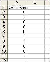
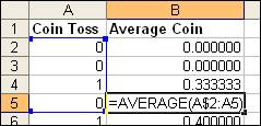
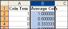
The first ten coin tosses

  1. Enter “Average Coin” in cell B1

  2. Click on cell B2 and enter:
        =average(a$2:a2)

  3. Drag B2’s fill handle down to cell B11. This is the same as using copy and paste to duplicate the formula.


  1. Boldface cells A1 and B1

    Your worksheet should look something like the one to the right. It shows the results of ten coin tosses and the average after each toss.

  2. How does the Average Coin formula in column B work? Why is there just one “$?

    Click on cell B5. The formula =AVERAGE(A$2:A5) calculates the average of cells A2 through A5.

    Click on cell B6. The formula =AVERAGE(A$2:A6) calculates the average of cells A2 through A6.

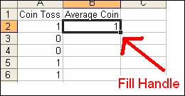
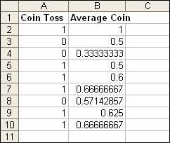
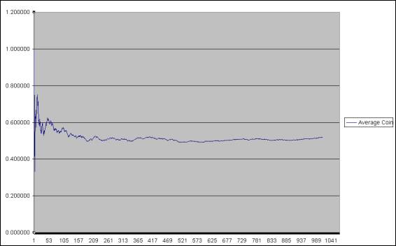
The “Average Coin” column is the average of all previous tosses

Cell B5 contains the average of cells A2 through A5

Excel created these formulas when you entered a formula in cell B2 and dragged it down in step 10.

The first cell reference is always A$2 because we want the AVERAGE calculation to start at the top of column A. The $ tells Excel not to change the “2” in the cell reference when you copy and paste the formula. This is an absolute cell reference.

The second cell reference is A5 in cell B5, A6 in cell B6, A7 in cell B7, and so on. There is no $ so Excel adjusts the row number when you cut and paste. This is a relative cell reference.

When you copy and paste the entire formula, each copy computes the average of all the coin flips starting from the first flip (cell A2) to the coin flip in the row that you paste to. After ten coin flips, the average in the example above is 0.66666667.

Part B – The RAND function

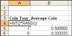
So, you’ve recorded ten coin tosses. You have a “running average” of the tosses. Now you’ll do at least 990 more coin tosses. Really! But the computer is going to do the coin tossing.

RAND is an Excel function that returns a random number that is greater than or equal to 0 and less than 1. For example: 0.12523, 0.938923, and 0.23923. With a little math, we can use RAND to randomly get either a 0 or a 1, and nothing in between.

Look at:

     =2*RAND()

This doubles the normal RAND function and returns a random number greater than or equal to 0 and less than 2. For example: 1.3923, 0.4239, etc. We want only whole numbers, so we use the INT function, which strips off the part to the right of the decimal point. For example, INT(1.5232) returns 1. So:

=INT(2*RAND())

returns either 0 or 1 with equal probability, just like flipping a coin.

 
You’ll use the RAND function in the next part. Don’t worry if you don’t quite understand this formula. It’s really a little bit of computer programming and thinking in this way may be new to you.


Part C – Lots of random numbers

  1. Click on cell A2

  2. Enter:
        =int(2*rand())

    The result of this formula is the same as flipping a coin.

  3. Click on the cell range A2:B2. Drag the fill handle of the two cells down at least to row 1000. The further down you drag the mouse the faster Excel will move the worksheet in the window.

RAND returns a number between 0 and 1

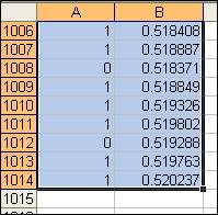
Drag columns A and B down past 1000

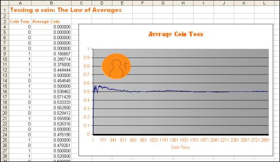
Part D – Charting the moving average

  1. Select column B by clicking on the letter “B” in the gray area at the very top of the Excel worksheet.

  2. Click the Insert menu and click Chart

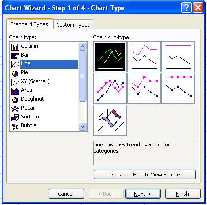
Select the entire column


  1. Choose a line chart with no point markers and click Finish

  1. Click Finish. You should see a chart appear on top of your spreadsheet. Move the chart so you can see both the chart and the first few coin flips of the spreadsheet.

    Notice how the Average Coin value changes on the graph. What number does the average tend towards?

  1. Right click on the y axis (the left edge of the chart) and choose Format Axis. You may need to try it a few times before you click on exactly the right place and get this menu.

  2. Click on the Scale tab and set Maximum to 1. Now your graph will show a grid line at 0.5. This will make the average coin value more obvious.

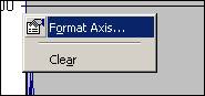
Right click exactly on the left edge of the chart
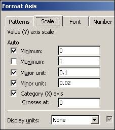
Change Maximum to 1


  1. Click on a blank cell in the spreadsheet (cell C2, for example). Press the Del key on your keyboard. Watch what happens to the graph.

    Deleting a blank cell is enough for Excel to regenerate all of the random number and give you an entirely new set of coin flips. Notice how the graph changes entirely and how different each set of coin flips is.

  2. Change the fonts or the formatting. Add a title. Add some art work. Have fun!